What is Bandwidth in an Oscilloscope? The Unseen Gatekeeper of Measurement Accuracy
I. Introduction: The Critical Role of Oscilloscope Bandwidth in Modern Engineering
In the contemporary landscape of high-speed digital design, complex embedded system development, and advanced automotive diagnostics, the integrity and reliability of diagnostic instrumentation are non-negotiable. The single most significant technical specification dictating the fidelity and accuracy of measurements derived from an oscilloscope is its bandwidth.1 If an oscilloscope fails to possess sufficient bandwidth, the resulting measurements will inherently be inaccurate, leading to compromised data, misleading results, and ultimately, flawed design decisions.2
The professional consensus among R&D technicians and electrical engineers is that bandwidth is the first and most vital characteristic to consider when selecting an oscilloscope.1 This determination moves far beyond simply comparing raw numbers. A comprehensive understanding requires detailing the technical mechanisms, the critical relationship between bandwidth and rise time, and the system constraints imposed by factors such as sampling rate and internal filtering architectures. This analysis aims to serve as a definitive guide, explaining not only what bandwidth is, but fundamentally why ignoring its limitations jeopardizes signal acquisition across all engineering applications.2
II. Deconstructing the Definition: The Physics of Oscilloscope Bandwidth
The concept of bandwidth in an oscilloscope is rooted in the instrument's analog front-end design. Functionally, the oscilloscope’s input stage, which includes the front-end amplifier, behaves like a low-pass filter (LPF).1 This inherent physical characteristic dictates the maximum frequency content that the instrument can accurately pass and process.
The Standard Metric: The -3 dB Point
Oscilloscope bandwidth is formally defined by the frequency at which the signal power attenuation reaches 3 decibels (dB), commonly referred to as the $-3 \text{ dB}$ point.1 The front-end amplifier’s frequency response resembles this low-pass filter characteristic.1
For engineers working primarily with voltage signals, it is more useful to interpret this attenuation in terms of voltage reduction. A drop of $-3 \text{ dB}$ corresponds precisely to the point where the signal's voltage amplitude has been reduced to $0.707$ (or $1/\sqrt{2}$) of its sensitivity level measured at DC or the lowest AC frequencies.4
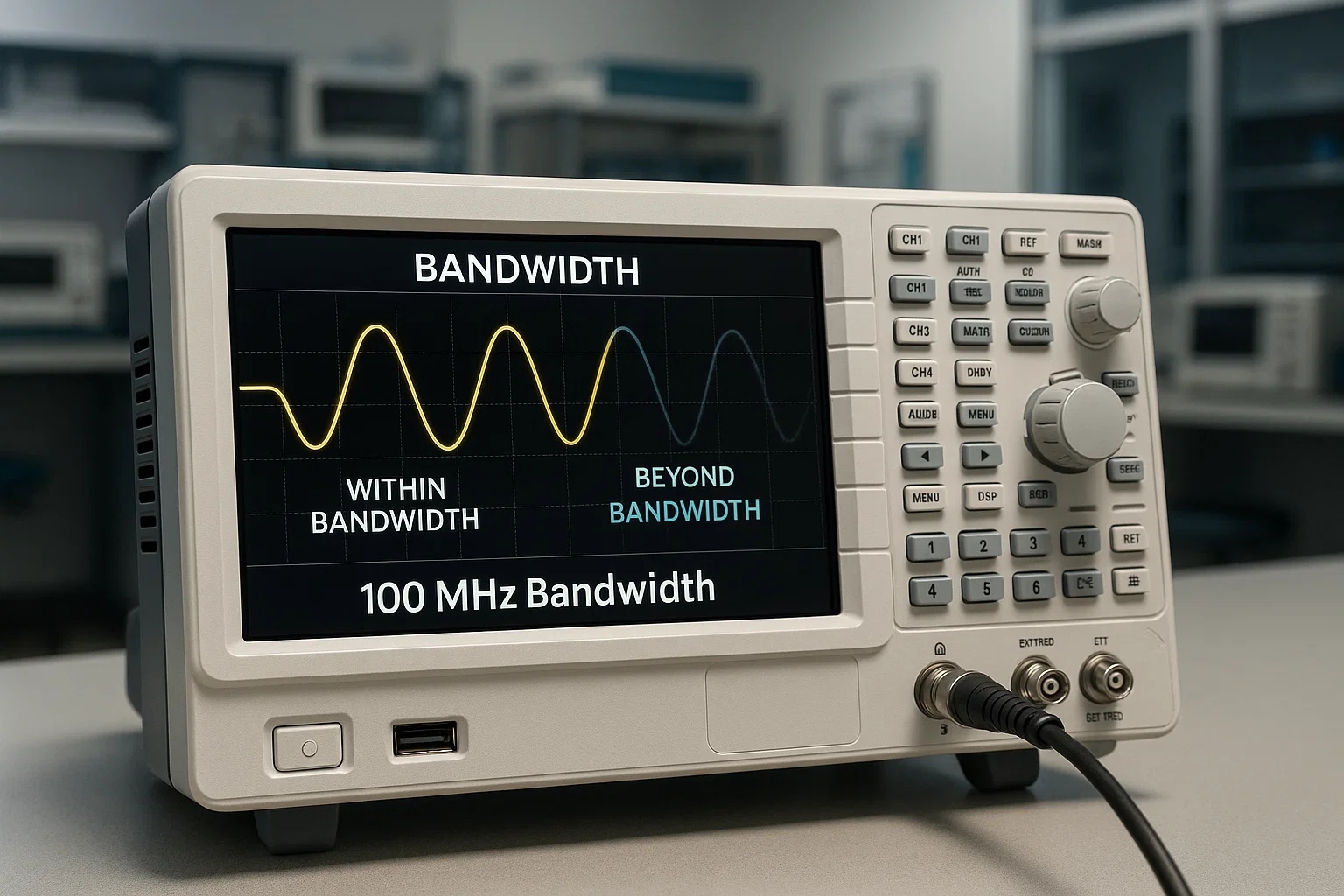
Critically, this standardized definition implies that at the rated bandwidth frequency, the oscilloscope is already displaying a voltage level that is approximately $30\%$ lower than the true input voltage amplitude.1 Beyond this $-3 \text{ dB}$ point, the oscilloscope's frequency response curve drops off rapidly, making any frequency content at or above this boundary unsuitable for making accurate amplitude or voltage level analyses.4
Implications of the Definition
The acceptance of a $-3 \text{ dB}$ (30% voltage) error standard for defining the bandwidth limit is a crucial point for professional instrument selection. The $-3 \text{ dB}$ point is a standardized tolerance rooted in historical power measurement (where $-3 \text{ dB}$ signifies half power). For voltage measurements in an oscilloscope, this tolerance establishes a usable boundary, but it critically dictates that engineers must select a bandwidth significantly higher than the signal frequency of interest to maintain an acceptable measurement error margin.
If the instrument is already introducing such significant inaccuracy at its specified maximum, it necessitates that the engineer select an oscilloscope with a bandwidth significantly higher than the highest frequency component of interest. The definition of oscilloscope bandwidth highlights that the specification is fundamentally an analog limitation, even for modern Digital Storage Oscilloscopes (DSOs).5 Therefore, the designated bandwidth is not a target frequency for precise measurement but rather an absolute boundary that, for meaningful data acquisition, must be exceeded by a wide margin.
III. The Crucial Relationship: Bandwidth and Signal Rise Time ($T_r$)
While the $-3 \text{ dB}$ point is essential for defining sinusoidal frequency limits, for analyzing digital signals (such as clock edges, data pulses, and fast transients), the speed of the signal transitions, known as the rise time ($T_r$), is the dominant constraint. Bandwidth and rise time are fundamentally linked through an inverse proportionality.6
The Bandwidth-Rise Time Rule and the K Factor
This inverse relationship is quantified by a core equation that allows engineers to determine the minimum required bandwidth based on the signal’s fastest edge:
$${f_{BW}} = \frac{K}{T_r}$$
In this formula, $f_{BW}$ is the bandwidth in Hertz, $T_r$ is the signal’s rise time in seconds, and $K$ is the proportionality constant, which is a key technical specification dependent entirely on the internal frequency response (filter design) of the oscilloscope.6
The value of $K$ varies depending on the instrument’s specific filter architecture and bandwidth capability 7:
-
Gaussian Response ($f_{BW} < 1 \text{ GHz}$): Oscilloscopes in this range typically feature a Gaussian frequency response and utilize a $K$ value of approximately $0.35$.6
-
Maximally-Flat Response ($f_{BW} > 1 \text{ GHz}$): High-end oscilloscopes often use a maximally-flat response, resulting in a higher $K$ value, generally falling between $0.40$ and $0.45$.7
For example, if a signal has a rise time of $700 \text{ picoseconds}$ ($0.7 \text{ nanoseconds}$), the required bandwidth using the standard Gaussian rule ($K=0.35$) is $500 \text{ MHz}$ ($0.35 / 0.7 \times 10^{-9} \text{ s}$).6
System Integrity and the K-Factor Bridge
The variation in the $K$ factor is a significant technical detail. The higher $K$ values associated with maximally-flat responses reflect a superior filter design that allows the oscilloscope to maintain a flatter passband before cutting off sharply.3 This efficiency means that for a given rise time, a higher-bandwidth scope with a Maximally-Flat filter can potentially provide a more accurate measurement than one relying on the simpler Gaussian model.
A critical system-level consideration is that the calculated rise time rule applies only to the oscilloscope's bandwidth. The actual rise time measured is the result of the entire measurement system (oscilloscope and probe). An inadequate probe can possess a slower rise time, dominating the system’s overall $T_r$ and neutralizing the benefits of a high-bandwidth instrument.8 Therefore, selecting a probe matched to the oscilloscope's capabilities is mandatory for preserving signal integrity.
Fundamental Oscilloscope Bandwidth Rules
| Concept | Definition/Formula | Source/K Factor |
| Bandwidth ($f_{BW}$) | Frequency at which sensitivity drops by 3 dB (70.7% voltage). |
Standard Definition 1 |
| Rise Time Rule | $f_{BW} = K / T_{r}$ |
Core Relationship 6 |
| K Factor (Gaussian) | $K \approx 0.35$ |
Typical for $f_{BW} < 1 \text{ GHz}$ 6 |
| K Factor (Maximally-Flat) | $K \approx 0.40 - 0.45$ |
Typical for $f_{BW} > 1 \text{ GHz}$ 7 |
| Accuracy Rule | Recommended $f_{BW} \geq 5 \times f_{signal}$ | Ensures capture of necessary harmonics. |
IV. The Design Engine: Understanding Oscilloscope Frequency Response Architectures
For rigorous test and measurement, knowing only the raw bandwidth specification is insufficient. Engineers must comprehend the instrument’s internal filter response curve, as this architecture determines how signals are attenuated and processed near the functional bandwidth limit.3 Oscilloscopes primarily utilize one of two frequency response architectures, each presenting distinct technical trade-offs.
1. Gaussian Frequency Response
The Gaussian response is characteristic of instruments with bandwidth specifications generally $1 \text{ GHz}$ and below.3 This architecture exhibits a gradual, slow roll-off. Attenuation often begins significantly early, at approximately one-third of the specified $-3 \text{ dB}$ frequency.3
The slow roll-off of the Gaussian filter means that in-band signals (below $f_{BW}$) begin degrading sooner. Although scopes with a Gaussian response typically attenuate out-of-band signals less aggressively than other types, the sacrifice in in-band flatness means they are less suitable for applications demanding extreme amplitude accuracy across the full specified bandwidth.3
2. Maximally-Flat Frequency Response (Brick Wall)
Maximally-flat responses are employed by high-end oscilloscopes, particularly those specified above $1 \text{ GHz}$.3 This design prioritizes an extremely flat amplitude response across the usable frequency band, resulting in minimal signal attenuation below the $-3 \text{ dB}$ limit. This superior flatness is followed by a sharp, rapid roll-off near the defined bandwidth frequency.3
The maximally-flat response delivers superior in-band amplitude accuracy because it attenuates signals less than a Gaussian scope within the defined operational range.3 This improved flatness is essential for advanced signal integrity analysis. The improved filter quality, capable of maintaining the frequency response closer to the limit, directly correlates with the use of the higher $K$ factor ($0.40-0.45$) in rise time calculations.7
The Accuracy and Attenuation Trade-Off
The transition between Gaussian and Maximally-Flat filtering reflects the industry’s need for greater precision in measuring high-order harmonics on modern, fast digital systems. The maximally-flat response ensures the preservation of signal amplitude further into the usable band, optimizing for accuracy. Conversely, the Gaussian response sacrifices some in-band flatness for a simpler roll-off profile. If a design requires guaranteeing sub-percentage amplitude accuracy, a Maximally-Flat scope is necessary because the signal amplitude is preserved closer to the bandwidth limit; a Gaussian response introduces unacceptable attenuation too early.3
V. The High Cost of Compromise: Signal Distortion from Insufficient Bandwidth
When an oscilloscope's bandwidth is inadequate, the resulting measurement error extends far beyond simple amplitude reduction; it fundamentally distorts the signal’s characteristics, compromising the validity of the entire analysis.
Waveform Integrity and Harmonic Attenuation
Complex waveforms, such as square waves or pulses, are composed of a fundamental frequency and a series of odd-order harmonics, as described by Fourier analysis. Accurate reproduction requires the instrument to capture not just the fundamental, but several of these high-order frequency components.10
If the oscilloscope bandwidth is insufficient, the instrument heavily attenuates or eliminates the higher frequency harmonics, leading to severe signal degradation.10 This phenomenon results in easily identifiable visual errors: square waves appear "rounded," and fast pulse edges are "smeared," or slowed down.10 This distortion leads directly to inaccurate measurements of crucial parameters like pulse width and signal rise time.10
The Two Critical Forms of Distortion
Insufficient bandwidth induces two distinct types of measurement error:
-
Amplitude Distortion: This is the direct attenuation of the signal's peak voltage, as defined by the $-3 \text{ dB}$ drop at the bandwidth limit. This leads to incorrect measurements of voltage levels ($V_{peak}, V_{pp}$), potentially misrepresenting power rails or signal amplitudes.1
-
Phase Distortion: This subtle error is particularly dangerous in digital systems. Insufficient bandwidth causes a shift in the phase relationship between the different frequency components (harmonics) of the signal.10 This phase shift introduces critical timing errors, such as jitter, by skewing the perceived timing of the rising and falling edges. In systems relying on precise clock synchronization or serial communication buses, phase distortion fundamentally invalidates timing analysis and leads to data errors.
The potential for phase distortion means that an inadequate bandwidth compromises timing integrity just as severely as it compromises voltage accuracy. An embedded systems engineer relying on the oscilloscope to verify a high-speed clock edge or data transition must ensure the bandwidth is high enough to prevent this phase shift, thereby ensuring the displayed pulse width and jitter characteristics are accurate.10
VI. Bandwidth in the Digital Age: Interplay with Sampling Rate (DSOs)
Digital Storage Oscilloscopes (DSOs) introduce a dual constraint on measurement: the analog bandwidth ($f_{BW}$) and the digital sampling rate ($R$). Both specifications must be sufficiently high to ensure signal fidelity.
The Necessity of Sampling Rate and Aliasing
The sampling rate ($R$ in Samples per second, Sa/s) determines the number of data points captured per second. If the rate is too low relative to the signal frequency, the instrument fails to accurately digitize the waveform, leading to aliasing. Aliasing occurs when the scope digitally reconstructs a false, lower-frequency signal, resulting in highly misleading trace representations.11
Linking Analog Bandwidth and Digital Sampling Rate
The required margin between the analog bandwidth and the sampling rate depends critically on the type of analog filter response employed 3:
For instruments utilizing a Gaussian frequency response, the slower roll-off requires a larger margin to prevent aliasing. The real-time sampling rate should be approximately 4 to 5 times the oscilloscope bandwidth ($R \geq 4-5 \times f_{BW}$).11
For oscilloscopes with a high-performance Maximally-Flat response, the sharper, more controlled roll-off allows for a lower multiplier. A rate of approximately 2.5 times the oscilloscope bandwidth ($R \geq 2.5 \times f_{BW}$) is often sufficient to maintain accuracy and prevent aliasing.11
The Crux of Digital Measurement
High bandwidth cannot rectify poor sampling rate, and a high sampling rate cannot compensate for low analog bandwidth. If the sampling rate is insufficient, the instrument produces aliased traces, rendering the high bandwidth capacity unusable. Conversely, low analog bandwidth simply prevents the signal energy from being captured in the first place.
For reliable digital measurements, the maximum frequency component should generally be limited to $f_{BW}/3$.11 This conservative limit accommodates the $70.7\%$ amplitude drop and provides the necessary margin for accurate digital reconstruction. This interaction demonstrates that the choice of analog filter architecture dictates the overall DSO architecture and necessary sampling rate overhead required for effective operation.
DSO Sampling Rate Guidelines for Aliasing Prevention
| Filter Type | Bandwidth Range | Recommended Sample Rate (R) | Technical Rationale |
| Gaussian |
Typically < 1 GHz 3 |
R $\geq 4 - 5 \times f_{BW}$ 11 |
Compensates for slow roll-off; higher margin needed to define bandwidth limit. |
| Maximally-Flat |
Typically > 1 GHz 3 |
R $\geq 2.5 \times f_{BW}$ 11 |
Sharper roll-off allows for a smaller multiplier while maintaining accuracy. |
VII. Selection Guidelines: Choosing the Right Oscilloscope Bandwidth for Your Application
Selecting the appropriate bandwidth is a systematic process that combines two core technical principles: the accuracy rule for signal frequency content and the rise time rule for digital transitions.
Principle 1: The General Accuracy Rule (5x Rule)
While basic signal tracing might accept a bandwidth three times the maximum fundamental signal frequency ($3 \times f_{max}$) 11, professional applications demanding high fidelity should adopt the more conservative $5 \times$ rule. It is recommended that the minimum required oscilloscope bandwidth ($f_{BW}$) be at least five times the maximum fundamental signal frequency component. This ensures the capture of up to the 5th harmonic, which is vital for maintaining square wave integrity and guaranteeing high-quality waveform reproduction.
Principle 2: The Digital Rise Time Rule
For high-speed digital analysis, the rise time rule (Section III) is the dominant factor. The required $f_{BW}$ must be calculated based on the fastest signal edge (shortest $T_r$) anticipated, utilizing the correct $K$ factor ($0.35$ or $0.40-0.45$) based on the instrument's design.7 The professional standard dictates using the rise time method for digital signals and then applying an additional accuracy margin to ensure measurement fidelity.
Application-Specific Mandates
Bandwidth requirements are dynamically escalating across several major engineering domains:
Embedded Systems and Clocking
Modern digital hardware requires sufficient bandwidth to capture the fast edges inherent in modern logic families.7 The bandwidth requirement is driven by the shortest $T_r$ in the system, ensuring that digital timing verification (e.g., jitter analysis, setup and hold times) can be performed without introducing measurement-induced distortion.
Advanced Automotive Diagnostics
The automotive diagnostic market is experiencing robust growth fueled by the rapid expansion of complex electronic systems, including Advanced Driver-Assistance Systems (ADAS) and Electric/Hybrid Vehicles (EV/HEV).12 These systems rely on intricate high-speed serial communication protocols and sophisticated switching components, necessitating high-fidelity oscilloscopes capable of analyzing complex electrical signals. The need to diagnose subtle faults in these systems directly mandates the adoption of instruments with higher bandwidths and improved signal fidelity.12 This market evolution confirms that high bandwidth is increasingly necessary for professional vehicle diagnostics and fault isolation.
VIII. Conclusion: Prioritizing Bandwidth for Measurement Certainty
Bandwidth defines the oscilloscope's operational envelope, established by the $-3 \text{ dB}$ attenuation point, which limits the usable frequency range. This specification is intrinsically linked to the ability to measure signal rise time accurately via the $K$ factor, and it governs the required digital sampling rate needed to prevent signal aliasing.
For accurate, reliable measurements—especially in demanding fields such as high-speed digital design or advanced automotive diagnostics—engineers must treat oscilloscope bandwidth as the non-negotiable cornerstone of their test bench. Compromising on this fundamental specification guarantees data integrity errors, including amplitude attenuation, edge smearing, and phase distortion, which are detrimental to timing verification.2 The rigorous selection process demands applying both the rise time calculation for fast edges and the $5 \times$ accuracy rule for frequency content, ensuring the chosen instrument captures the true nature of the signal and provides verifiable measurement certainty.